An Evolution of Learning to Rank
First Thing First
Enigmas of the universe
Cannot be known without a search
— Epica, Omega (2021)
In The Rainmaker (1997), the freshly graduated lawyer Rudy Baylor faced off against a giant insurance firm in his debut case, almost getting buried by mountains of case files that the corporate lawyers never expected him to sift through. If only Rudy had a search engine that retrieves all files mentioning suspicious denials and ranks them from most to least relevant, the case prep would’ve been a breeze.

Search process overview: Indexing, matching, ranking (Relevant Search)
For a holistic view of search applications, I highly recommend the timeless Relevant Search (repo). Raw documents go through analysis to get indexed into searchable fields (e.g., case name, case year, location, etc.). At search time, a user-issued query (e.g., “leukemia”) undergoes the same analysis to retrieve matching documents. Top documents are ranked in descending order of relevance before being returned. This post focuses on ranking, especially learning to rank (LTR).
Problem Formulation of LTR
“Ranking is nothing but to select a permutation $\pi_i \in \Pi_i$ for the given query $q_i$ and the associated documents $D_i$ using the scores given by the ranking model $f(q_i, D_i)$.” — A Short Introduction to LTR, Li (2011)
LTR learns how to sort a list of documents retrieved for a query in descending order of relevance. During training, it sees many instances of how documents are ordered for different queries; once trained, LTR can order new documents for new queries, using a learned function $f(q, D)$ that scores documents $D$ given a query $q$.

A single training instance consists of the following components:
- A query $q_i$ and a list of documents $D_i = \{d_{i, 1}, d_{i, 2}, …, d_{i, n}\}$;
- The relevance score of each document given the query $Y = \{y_{i, 1}, y_{i, 2}, …, y_{i, n}\}$;
- A feature vector for each query-document pair, $x_{i, j} = \phi(q_i, d_{i, j})$
Even if you don’t work at a company with search engines, you can still play with publicly available LTR datasets, such as the famous The Yahoo! Learning to Rank Challenge dataset. More recently at NeurIPS 2022, Baidu Search released a dataset with richer features and presentation information. Try them out!
What is the “Right” Order?
Evaluation Metrics
What makes LTR special is that it penalizes predictions that lead to “out-of-order” document ranking compared to the “ideal ranking”, rather than getting each individual document’s score right. Ideal ranking is usually determined by human judgments (classic 5-point scale: “perfect”, “excellent”, “good”, “fair”, “bad”) or user engagement (e.g., conversion: 3, click: 2, impression: 1).

In the example above, the search engine ranks a less relevant document above a more relevant one, so it’s not perfect. A common ranking metric that takes all relevant documents and their ordering into account is Normalized Discounted Cumulative Gain at top k results (nDCG@k), which can be computed as the following:
- DCG: Given a ranking for query $q_i$, we can compute a Discounted Cumulative Gain for top k documents (DCG@k), $DCG_k = \sum_{j}^{k} \frac{\mathrm{rel_{i,j}}}{\log_2 (j + 1)}$, where the relevance label of the document at position $j$ is its “gain”, and $\log_2 (j + 1)$ is a position discount function. In this case, $DCG_3 = \frac{5}{\log_2 (1 + 1)} + \frac{3}{\log_2 (2 + 1)} + \frac{4}{\log_2 (2 + 1)} \approx 9.02$.
- IDCG: We can compute DCG@k for the ideal order, or “Ideal Discounted Cumulative Gain at k (IDCG@k)”. Here, $IDCG_3 = \frac{5}{\log_2 (1 + 1)} + \frac{4}{\log_2 (2 + 1)} + \frac{3}{\log_2 (2 + 1)} \approx 8.89$.
- nDCG: The ratio of DCG@k and IDCG@k is nDCG@k: $nDCG_k = \frac{DCG_k}{IDCG_k}$.
In this example, $nDCG_3 = 8.89 / 9.02 \approx 0.98$, which is just short of perfect (1). If we completely reverse the document order from the ideal order, the result is still not bad: $DCG_3 = \frac{3}{\log_2 (1 + 1)} + \frac{4}{\log_2 (2 + 1)} + \frac{5}{\log_2 (2 + 1)} \approx 8.02$ and $nDCG_3 = 8.02 / 9.02 \approx 0.89$. This is because irrelevant results (1 or 2 ratings) didn’t even make it to top k. However, what if top k results are all bad? nDCG@k would still be 1 as long as the model ranks documents in the same order as relevance labels would. nDCG@k measures the goodness of ranking, but even perfect ranking cannot save search relevance if bad documents dominate top k results due to flawed retrieval/first-pass ranking.
When we don’t have fine-grained relevance ratings but only 0 (“Not Relevant”) / 1 (“Relevant”) labels, we can use other ranking metrics that fall under 2 categories:
- Order-unaware metrics: Easy to compute but document order is ignored
- R@k (recall @k): # of relevant docs in top k / # of relevant docs
- P@K (precision @K): # of relevant docs in top k / k
- Order-aware metrics: What is search, if not to order results?
- MRR (mean reciprocal rank): On average, how early the 1st relevant doc shows up 👉 $\frac{1}{n}\sum_{1}^{n}\frac{1}{\mathrm{rank}_i}$, where $q_i$ is a query in an eval query set of size $n$, and $\mathrm{rank}_i$ is the rank of the 1st relevant doc for $q_i$
- MAP@k (mean average precision @k): For each query, we can compute its average precision across top k (AP@k), weighted by binary relevance @k 👉 $AP_k = \frac{\sum_{1}^k(P@k \cdot \mathrm{rel}_k)}{\sum_1^k \mathrm{rel}_k}$. AP@k across the eval set is then the MAP@k.
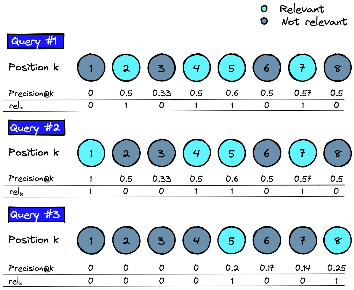
MAP@k, Evaluation Measures in Information Retrieval by Pinecone
Ranking Loss
Using nDCG to measure LTR performance, the true loss function is $L(F(\mathbf{x}), \mathbf{y}) = 1.0 - nDCG$, where $F(\cdot)$ is a function mapping from a list of feature vectors $\mathbf{x}$ to a list of scores, and $\mathbf{y}$ is a list of true scores. The sorting operation in nDCG makes the true loss non-differentiable at times. Below are 3 types of surrogate losses.
-
Pointwise: Predict how relevant each doc is for a given query
- General form: $L'(F(\mathbf{x}), \mathbf{y}) = \sum_{i=1}^n (f(x_i) - y_i)^2$; same as a regular regression model (or binary classification, or ordinal regression models)
- Motivation: If we predict each document’s relevance w.r.t. the query well, hopefully we can get an ideal order for free
- Drawbacks: Doesn’t optimize for ranking at all — small predictions errors on individual docs may result in a completely out-of-order list; doesn’t leverage relationships between docs retrieved for the same query
-
Pairwise: Predict which among a pair of docs is more relevant for query
- General form: $L'(F(\mathbf{x}), \mathbf{y}) = \sum_{i=1}^{n-1} \sum_{j=i+1}^{n} \phi (\mathrm{sign}(y_i - y_j), f(x_i) - f(x_j))$, which makes the score of a more relevant doc higher, and the score of a less relevant doc lower for each given query
- Motivation: If we can predict the better doc among each pair (e.g., A > B, B > C, A > C), we can recover the best global order (A > B > C)
- Drawbacks: Doesn’t optimize for global ranking — if we swap a pair (e.g., A < B, B > C, A > C), then the global ranking is wrong (B > A > C)
- History: Chris Burges from Microsoft proposed 3 methods for pairwise LTR: RankNet, LambdaNet, and LambdaMART (used by LightGBM)
-
Listwise: Predict the best permutation of docs for a query — like the true loss
- General form: $L'(F(\mathbf{x}), \mathbf{y}) = \exp(-nDCG) = \sum_{i=1}^m (E(\pi^*_i, \mathbf{y_i}) - E(\pi_i, \mathbf{y_i}))$, where $\pi_i$ is the permutation generated by labels and $\pi^*_i$ by model scores
- Motivation: Get the global ranking right in a straightforward way
- Drawbacks: Computationally expensive to enumerate all doc permutations and far more complicated to implement than pointwise or pairwise approaches
- History: Later, Google researchers proposed a generalized framework LambdaLoss, which encompasses pointwise, pairwise, and listwise approaches
Rank without Learning
How do we learn that $f(q_i, D_i)$ function? This is a loaded question because this function is not always learned. LTR was only popularized in the last 15 years or so, whereas traditional search engines rely on the textual match between a query and documents to determine document relevance. Due to their simplicity, these methods are still used by modern search engines to retrieve top N documents to re-rank.
TF-IDF
When searching on Netflix, for example, the query “rebecca” could match a movie’s title (e.g., Hitchcock’s Rebecca), cast (e.g., actress Rebecca Ferguson), or description (e.g., protagonist named Rebecca appeared in the summary). Queries and document fields can all be represented by TF-IDF vectors — each element in the vector represents a token in the “vocabulary” and the value is 0 if the given token is absent or the product of “TF” (term frequency: how many times the token appears in the corpus) and “IDF” (inverse document frequency: 1 / in how many documents does the token appear). The dot product between a query’s and a field’s TF-IDF vectors measures their closeness (higher is better), which is used to rank documents.
Fields can have different weights — perhaps, a title match is 3 times more important than a cast match, and 10 times more important than a description match. These weights usually come from heuristics and are tuned by observing search defects.
BM25
Whether “Rebecca” appears once in a document field or 10 times, the dot product between the two would be the same. A family of ranking functions, BM25, scores each document $D$ by counting how many times terms $q_1, \ldots, q_n$ in the query $Q$ appear in it (notations differ from previous sections: $q_i$ is a query term, not the whole query).
“25” denotes the 25th version and even it takes many forms. A classic instantiation is $\mathrm{score}(D, Q) = \sum_{i=1}^{n}\mathrm{IDF}(q_i)\cdot \frac{f(q_i, D)\cdot (k1 + 1)}{f(q_i, D) + k_1 \cdot (1 - b + b \cdot \frac{|D|}{\mathrm{avgdl}})}$, where $\mathrm{IDF}(q_i)$ is the inverse document frequency of the query term $q_i$, $f(q_i, D)$ is the frequency of $q_i$ in $D$, $|D|$ is the token-level document length, and $\mathrm{avgdl}$ is the average document length across the corpus. $k_1$ and $b$ are free parameters with typical values $k_1 \in [1.2, 2.0]$ and $b = 0.75$.
Learning to Rank
TF-IDF and BM25 are driven by “magical numbers”: How do we find the best document field weights? Where do free parameters $k_1$ and $b$ in BM25 come from? Moreover, the two or similar methods treat relevance as an inherent, static property between a query and a document. However, relevance also depends on who is searching in what context — I’m a big Hitchcock fan so Rebecca (1940) is likely what I want whereas you want to watch another movie starring Rebecca Ferguson coming from Dune and Mission Impossible. Machine learning is a natural choice to leverage query, document, user, and context features to systemically optimize for search relevance.
Traditional ML
When using pointwise loss, ranking can be framed was a regression (predict relevance scores) or a classification (predict click probabilities) problem, for which any regression or classification models work. As discussed, this overly simplified approach doesn’t optimize for document ordering, so we won’t go into depth here.
RankSVM is an early linear model that optimizes for pairwise loss. Today, pairwise LTR based on Gradient Boosted Decision Trees (GBDT) is by far the most popular — LambdaMART and its LightGBM implementation are widely used in commercial search engines and, until recently (Qin et al., 2021), outperformed all neural rankers.
LambdaMART uses the LambdaRank gradient for pairwise loss, $\log(1 + \exp(-\sigma(s_i - s_j)))|\Delta \mathrm{nDCG}|$, which, at its core, is a position-aware version of binary log loss.
- Pairwise ranking as binary classification: Pairwise loss converts document ranking into $k \choose 2$ binary classification problems, where $k$ is the number of top documents to re-rank for the given query. Say document $i$ is more relevant than $j$, how likely will the model rank $i$ above $j$? This probability $\mathrm{Pr}(i > j)$ is given by the logistic function, $\frac{1}{1 + \exp(-\sigma(s_i - s_j))}$ — if $s_i = s_j$, the model has a fifty-fifty chance of guessing right; if the diff is in the right/wrong direction, then the model has a higher/lower probability of ranking the pair in the correct order.
- Note: In LightGBM, the hyperparameter $\sigma$ defaults to 1
- Injecting position information with nDCG: Swapping the order of $i$ and $j$ gives us 2 ranked lists — the nDCG difference between the 2 lists is given by $|\Delta \mathrm{nDCG}|$. This term captures our intuition that swapping positions 1 and 2 has more severe consequences than, say, swapping positions 9 and 10.
- LambdaRank gradient: $\lambda_{ij}$ is simply the product of $\log \mathrm{Pr}(i > j)$ and $|\Delta \mathrm{nDCG}|$.
Like other GBDT models, LambdaMART assigns higher weights to document pairs with higher loss, so that the model will focus on such pairs in later iterations. While deep learning has become the gold standard in fields such as natural language processing (NLP) and computer vision (CV), GBDT still dominates search ranking, especially on tabular data. One reason is that GBDT is robust to feature scales — the absolute values don’t matter, so long as the relative ordering is correct — whereas neural nets require careful feature normalization and scaling to learn. Another reason is that in academia, LTR benchmarks are not big enough for DL to shine, yet in industry, search is a surface with strict latency requirements and DL models can have much higher latency than famously fast GBDT models such as LightGBM.
Deep Learning
It’s interesting that in CV, DL replaced non-DL methods (e.g., hierarchical Bayes) as the mainstream after the ImageNet breakthrough in 2012, whereas LTR saw a transition from DL (RankNet (2005), LambdaRank (2007)) to non-DL (LambdaMART (2010)). Early neural LTR typically uses a feed-forward network with fully connected layers, which doesn’t play to DL’s strength: Learning higher-order feature interactions. Moreover, early neural LTR didn’t put much focus on feature transformation, which can profoundly impact neural nets. Google researchers (2021) demonstrated that using newer architectures on transformed data, neural LTR was able to beat LightGBM.
- Normalization: The feature vector $\mathbf{x}$ goes through “log1p” transformation, $\mathbf{x} = \log_e(1 + |\mathbf{x}|) \odot \mathrm{sign}(\mathbf{x})$, where $\odot$ is element-wise multiplication.
- Gaussian noise: A random Gaussian noise is injected to every element of the feature vector $\mathbf{x}$, $\mathbf{x} = \mathbf{x} + \mathcal{N}(\mathbf{0}, \sigma^2 \mathbf{I})$, to augment input data.
- Multi-head self-attention: Documents in the ranked list are encoded with multi-head self-attention to generate a contextual embedding for each doc.
On Web30K and Istella benchmarks, the neural LTR outperformed LightGBM (still lost in the Yahoo! benchmark), showing DL is not inherently inferior for ranking.

Smashing benchmarks may not be so exciting if that’s all LTR can do — the Airbnb trilogy (2019, 2020, 2023) proved out the power of DL in commercial search engines. Not only did offline nDCG and online conversions increase, but DL allows ML engineers to shift the focus from Kaggle-style feature engineering to deeper questions about ranking: What’s the right objective to optimize for (multi-task, multi-objective learning)? How to better represent user/query/docs (two-tower architecture)?
Fully-Connected DNNs
“Deep learning was steep learning for us." — Haldar et al. (2019) @Airbnb
In 2016, the Search team at Airbnb saw a long spell of neutral experiments adding new features to GBDT models and turned to DL for breakthroughs. The journey took 2 years. The final model was a DNN with 2 hidden layers trained on LambdaRank loss:
- Input layer with 195 features
- 1st hidden layer with 127 fully connected RELUs
- 2nd hidden layer with 83 fully connected RELUs
- Output is scores of a pair of booked vs. unbooked listings
On the way to this seemingly straightforward model, many (failed) paths were tread.
- Architectural complexity: Deep NN outperformed bespoke simple NNs in this case
- Simple NN with pointwise loss: To validation the NN pipeline was production ready, the Airbnb Search team started with a simple NN that had a single hidden layer trained on the pointwise L2 regression loss: Booked listings were assigned a value of 1.0 whereas unbooked ones 0.0. The model created tiny gains in offline nDCG and online bookings.
- Simple NN with LambdaRank loss: Keeping the architecture the same while shifting to pairwise LambdaRank loss increased the gains.
- Simple NN with GBDT + FM inputs: The team experimented with a more complex structure where outputs from GBDT and factorization machine (FM) were fed as inputs to the NN with a single layer. The index of active leaf nodes from GBDT were used as categorical features whereas the predicted booking probability from FM were used as a numerical feature. While this model saw both offline and online improvements, it was a maintenance hell.

- Feature engineering: While Deep NNs are known for automatic feature extraction, they could still benefit from careful feature selection and transformations
- Do not use listing IDs: It is a common practice in DL to encode high-cardinality categorical features such as IDs as lower-dimensional embeddings and learn these embedding values via backpropagation. However, using listing IDs as a feature led to overfitting, because Airbnb has this unique problem that listings, by design, can only be booked at most 365 times a year, so the model doesn’t have much to learn about each listing.
- Examine feature distributions: NNs are sensitive to feature scales, so it’s standard practice to transform feature values into the $\{-1, 1\}$ range before feeding them to the model. Mostly normally distributed features were transformed into z-scores, $\frac{x - \mu}{\sigma}$. Features with power law distributions were log-transformed, $\log \frac{1 + x}{1 + \mathrm{median}}$. Plotting feature distributions also helped detect bugs such as monthly prices being logged as daily prices in some locations, breaking otherwise smooth distributions.
- Multi-task learning: Learning doesn’t always transfer the way you think it does
- Long views didn’t translate to bookings: As mentioned, bookings are far and few between, but long views occur much more frequently and are correlated with bookings. So perhaps a multi-task model trained to predict both long view and booking probabilities can transfer its learning from the former to the latter. Moreover, this may enable us to learn listing embeddings because now each listing has sufficient long views. However, this multi-task model hurt the online booking rate — a likely explanation is that listings users like to view but don’t book are often high-end stays with high prices, have long descriptions, or just look peculiar.

- Long views didn’t translate to bookings: As mentioned, bookings are far and few between, but long views occur much more frequently and are correlated with bookings. So perhaps a multi-task model trained to predict both long view and booking probabilities can transfer its learning from the former to the latter. Moreover, this may enable us to learn listing embeddings because now each listing has sufficient long views. However, this multi-task model hurt the online booking rate — a likely explanation is that listings users like to view but don’t book are often high-end stays with high prices, have long descriptions, or just look peculiar.
Airbnb’s journey has since inspired many companies to pursue the neural LTR path. DL isn’t just a fad, but it truly frees ML engineers from manual feature engineering and lets the model learn feature interactions and entity representations from data, and encourages deeper thinking about learning objectives and representations.
Two-Tower Architecture

Growing up, The Two Towers is the second installment of my favorite trilogy The Lord of the Rings — as it happens, it’s also the second in the Airbnb’s neural LTR journey, addressing the tricky issue of balancing relevance and listing prices.
At Airbnb, the final booking price often fell on the lower side of the median price on the search result page, suggesting many guests preferred a lower price than shown. Every method of directly enforcing a lower price hurt bookings, including:

- Remove price as a model feature and add it to output: $DNN_\theta (u, q, l_{\mathrm{no\,price}}) - \tanh(w \cdot \mathcal{P} + b)$, where $\mathcal{P} = \log \frac{1 + \mathrm{price}}{1 + \mathrm{price}_{\mathrm{median}}}$. The first term is the DNN output without the price feature, and the second term increases monotonically with price — all else being equal, more expensive listings will have lower scores and get down-ranked. This model reduced the average price but severely degraded bookings. An explanation is that price has interactions with many features — i.e., what’s considered expensive depends on the location, the number of guests/nights, the time of year, etc. — removing it led to under-fitting.
- DNN partially monotonic w.r.t. price: The team added price (more precisely $\mathcal{P}$) back as a feature and tweaked the DNN architecture so that the final output was monotonic with respect to price. However, like the previous approach, listings with absolute high prices were down-ranked, regardless of the context.

- Adding a price loss: Apart from predicting the booking probability, this version also predicted the price. The total loss is a linear combination of the booking loss and the price loss. This model didn’t generalize well online because it didn’t accurately predict the price of entirely new inventory.
The heart of is the problem is, the team just assumed “cheaper is better” when really the holy grail was “finding the right price for a trip”. Some guests like lavish places; bigger places and longer stays in hot destinations are naturally more expensive. To capture guest preferences and listing attributes, we need a good presentation of each entity, for which the two-tower architecture is a natural choice.
- Architecture: The model consists of a query-user tower and a listing tower

- Query-user tower: Has all query and user features — each query-user combination has an “ideal listing” (100-vector)
- Listing tower: Has all listing features as 100-vectors
- Training data: In typical contrastive representation learning, each training instance consists of a triplet of items — an anchor item, a positive example (same label as anchor), and a negative example (different labels from anchor). The goal of learning is to pull the positive example closer to the anchor and push the negative example away from the anchor in the embedding space. This case is slightly different: The triplet consists of a query-user combination, a booked listing, and an unbooked listing, not 3 listings. The goal is similar.
- Triplet loss: $\mathcal{L}_{\mathrm{triplet}} = \max(0, d(a,p) − d(a,n) + \mathrm{margin})$, where $d(a,p)$ is the distance between the anchor $a$ and the positive $n$, $d(a, n)$ the distance between $a$ and the negative $n$, and $\mathrm{margin}$ defines how much further $n$ needs to be from $a$ than $p$ needs to be from $a$. If $n$ is much further from $a$ than $p$ is, the loss will be 0; if both close to $a$ or $p$ is even further, the loss is positive.
- Inference: Trained on $\mathcal{L}_{\mathrm{triplet}}$, the model learns a 100-d dimension embedding of each query-user combination and each listing. At inference time, dot products between query-user and listing embeddings are used to score and rank listings.
While low price was not enforced by the two-tower model, the average price in search results decreased, without hurting bookings — by learning query/user/listing representations, the model found “the right price for the right trip”.
This paper additionally addressed 2 common issues in search engines in clever ways:
- Cold start: The team focused on cold-starting new listings. Rather than using magical numbers to boost new listings and decaying the boosting factor by # impressions and recency, the team build a model to infer missing engagement features for new listings (e.g., based on listings in the neighborhood) — after all, that’s the biggest difference between new listings and existing ones. The model resulted in a staggering 14% increase in new listing bookings.
- Position bias: Directly adding position as a feature and setting it to 0 at inference time may result in the model over-fitting to position. Adding a dropout (probabilistically setting some positions to 0) reduced over-fitting.
Multi-Task Learning
Most recently, the Airbnb Search team switched to a multi-task “Journey Ranker”, a new industry gold standard. The motivation came from a unique Airbnb user problem: Guests often go through a long journey (click $\rightarrow$ view listing details, or “long click” $\rightarrow$ visit payment page $\rightarrow$ request stay $\rightarrow$ pay) before booking, and it can be frustrating to have the host reject the booking or either party decides to cancel later on. The North Star of Airbnb Search is uncancelled bookings and the multi-task learner traces the long-winded journey to optimize for this goal.

Listing and context (user, query) features go through separate MLP layers to create embeddings, which are then fed to both the “base module” and the “twiddler module”:
- Base module: Predicts probability of the final positive outcome (uncancelled booking) by chaining probabilities of 6 positive milestones ($\mathrm{c}$: click; $\mathrm{lc}$: long click, $\mathrm{pp}$: payment page, $\mathrm{req}$: request, $\mathrm{book}$: booking, $\mathrm{unc}$: uncancelled booking) 👉 $p(\mathrm{unc}) = p(\mathrm{c}) \cdot p(\mathrm{lc} | \mathrm{c}) \cdot p(\mathrm{pp} | \mathrm{lc}) \cdot p(\mathrm{req} | \mathrm{pp}) \cdot p(\mathrm{book} | \mathrm{req}) \cdot p(\mathrm{unc} | \mathrm{book})$
- Hard parameter sharing: Representation is shared by all 6 task heads
- Final loss: Sum of each individual task $t$’s loss, $\mathcal{L}_{base} = \sum_t \mathcal{L}_t$
- Task loss: $\mathcal{L}_t = \sum_u \sum_s l_t (s|\theta) \cdot w_t$, where $u \in U$ is a user, $s \in S_u$ is a search by $u$, and $l_t (s|\theta)$ is a standard ranking loss. To prevent common tasks (e.g., clicks) from dominating the final loss, a weight $w_t$ is assigned to each task, which can be the inverse of ${p(\mathrm{unc} | t)}$ — the observed probability that there will be an uncancelled booking if the task is completed.
- Twiddler module: A booking could be cancelled by the user or by the host, which is not captured in the base module. The twiddler module is dedicated to predicting negative milestones, including host rejection, guest cancellation, and host cancellation. The outputs are 3 predicted probabilities.
- Why build this module: One reason is given — bookings can fail in multiple ways, yet the base module meshes them together and only predicts the final success probability. Moreover, negative milestones are rare — the authors found having a separate module was better for battling class imbalance.
- Final loss: Also sum of each individual task $t$’s loss, $\mathcal{L}_{twiddler} = \sum_t \mathcal{L}_t$
- Task loss: Binary classification loss for each of the negative milestones
The combination module combines outputs from the base and the twiddler modules to output a relevance score. It learns the weights used in the linear combination, $y_{combo} = y_{base} \cdot \alpha_{base} + \sum_{t \in twiddler} y_t \cdot \alpha_t$, while parameters in previous modules are frozen. The final loss of the multi-task learner is the sum of losses in the 3 modules.
The multi-task ranker simultaneously reduced cancellations and improved search relevance. Advantages compared to past Airbnb models predicting 0/1 booking labels:
- Quantity: Bookings are sparse, whereas data from earlier milestones are larger in quantity and informative to the final outcome
- Diversity: The model sees searches from a variety of bookers and non-bookers
- Intermediate predictions: Intermediate outputs may be used as stand-alone predictions or inputs to other models

One thing to note is that the Airbnb paper adopted hard parameter sharing, where a single input representation is shared by all tasks. If some tasks are not highly correlated, the model performance will be compromised. Researchers from YouTube published a paper using a Multi-Gate Mixture-of-Expert (MMoE) layer to determine which tasks should share parameters and which ones should not. Looking back, Airbnb’s first attempt at multi-task learning might have suffered from not highly correlated tasks (bookings vs. long views), for which MMoE could be a solution.

LLM Re-Rankers
“Ranking documents using Large Language Models (LLMs) by directly feeding the query and candidate documents into the prompt is an interesting (😂) and practical problem.” — Qin et al. (2023)
Ranking seems like a bad use case for LLMs since documents are enormous and relevance is personal and contextual. Upon second thought, why not — LTR was trained on human ratings before large-scale search logs and is still evaluated by humans.
Early attempts focused on pointwise (e.g., Liang et al. 2022) and listwise (e.g., Sun et al., 2023) prompting, which proved difficult for LLMs:

- Pointwise: The prompt asks LLMs to assign a relevance rating to each query-document pair. This approach is not logically sound. First of all, LLMs are unable to provide calibrated probabilities across prompts which we can use to sort documents in an optimal order. Secondly, some models (GPT-4) don’t output probabilities at all. Lastly, absolute probabilities are not even necessary for LTR, which relies on the relative probabilities of documents.
- Listwise: Asking LLMs to re-rank the document list seems to address all issues above; in reality, LLMs sometimes miss or repeat documents, generate nonsensical ordering, rank the same list differently when prompted again, or refuse to rank. So far, only GPT-4 does well but it’s cost prohibitive.
Pairwise prompting recently proposed by Google Search researchers led to a performance breakthrough. The LLM is given a pair of documents for each query and either prompted to choose the more relevant document (generation) or assign scores to both (scoring). To mitigate order effect, each pair is shown twice in reverse ordering.

To get the list order, the $O(N^2)$ brute-force solution is to rank all pairs (twice per pair, if we want to mitigate order effect). Efficient sorting algorithms such as Quicksort and Heapsort reduce time complexity to $O(N \log N)$. The sliding window approach does a single scan through the document list, swapping each consecutive pair iff LLM disagrees with the initial ranking, reducing time complexity to $O(N)$.

This model outperformed other GPT-based models, as well as BERT-based cross-encoder re-rankers at that time. Later models such as RankZepher were able to perform listwise ranking using smaller LLMs distilled from GPT 3.5/4 (is that even allowed? 😂). These LLM re-rankers are often compared to the BM25 baseline and other LLM re-rankers, but not GBDT or neural LTR. I guess when you have a small search engine (perhaps for a personal/startup project), it’s easier to get off the ground using an LLM re-ranker when GBDT and neural LTR can be quite data hungry.
Learn More
Papers
- Burges, CJC. (2010). From RankNet to LambdaRank to LambdaMART: An overview. Microsoft Research Technical Report.
- Haldar, M., Abdool, M., Ramanathan, P., Xu, T., Yang, S., Duan, H., … & Legrand, T. (2019). Applying deep learning to Airbnb search. SIGKDD.
- Haldar, M., Ramanathan, P., Sax, T., Abdool, M., Zhang, L., Mansawala, A., … & Liao, J. (2020). Improving deep learning for Airbnb search. SIGKDD.
- Joachims, T. (2006). Training linear SVMs in linear time. SIGKDD.
- Li, H. (2011). A short introduction to learning to rank. IEICE TRANSACTIONS on Information and Systems, 94(10).
- Pradeep, R., Sharifymoghaddam, S., & Lin, J. (2023). RankZephyr: Effective and robust zero-shot listwise reranking is a breeze! arXiv.
- Qin, Z., Yan, L., Zhuang, H., Tay, Y., Pasumarthi, R. K., Wang, X., and Najork, M. (2021). Are neural rankers still outperformed by gradient boosted decision trees?, ICLR.
- Qin, Z., Jagerman, R., Hui, K., Zhuang, H., Wu, J., Shen, J., … & Bendersky, M. (2023). Large language models are effective text rankers with pairwise ranking prompting. arXiv.
- Tan, Chun How, Austin Chan, Malay Haldar, Jie Tang, Xin Liu, Mustafa Abdool, Huiji Gao, Liwei He, and Sanjeev Katariya. Optimizing Airbnb search journey with multi-task learning. arXiv.
- Wang X., Li C., Golbandi, N., Bendersky, M., and Najork, M. (2018). The LambdaLoss framework for ranking metric optimization. CIKM.
- Yan, L., Qin, Z., Zhuang, H., Wang, X., Bendersky, M., & Najork, M. (2022). Revisiting two-tower models for unbiased learning to rank. SIGIR.
- Zhao, Z., Hong, L., Wei, L., Chen, J., Nath, A., Andrews, S., Kumthekar, A., Sathiamoorthy, M., Yi, X., and Chi, E., (2019). Recommending what video to watch next: A multitask ranking system. RecSys.
Blogposts
- Introduction to Learning to Rank by Kyle Chung (2019)
- The inner workings of the LambdaRank objective in LightGBM by Frank Fineis (2021)
- Contrastive Representation Learning by Lilian Weng
- Deep Multi-task Learning and Real-time Personalization for Closeup Recommendations by Pinterest (2023)
- Using LLMs for Search with Dense Retrieval and Reranking by Cohere (2023)